Chapter 4 Output Results
## Loading required package: limma## Loading required package: mgcv## Loading required package: nlme## Warning: package 'nlme' was built under R version 4.1.2## This is mgcv 1.8-38. For overview type 'help("mgcv-package")'.## Loading required package: genefilter## Loading required package: BiocParallelThe online tool outputs three figures to show the results after data normalization.
4.1 Boxplot
The boxplot shows the distribution of protein abundance for each sample. Figure 4.1 shows the boxplot of protein abundance for raw data, after median normalization and after quantile normalization. After data normalization, the distribution of protein abundance for each sample is more similar to each other.
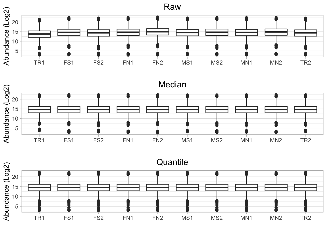
Figure 4.1: Boxpolt of protein abundance for each sample in a single batch (before and after normlization)
For data from multiple batches, the online tool takes data normalization for each batch first (Figure 4.2). The data within each batch is similar to each other after quantile normalization in each batch. However, samples in batch 1 have higher value than the samples in batch 2. Batch effect correction is necessary before further data analysis.
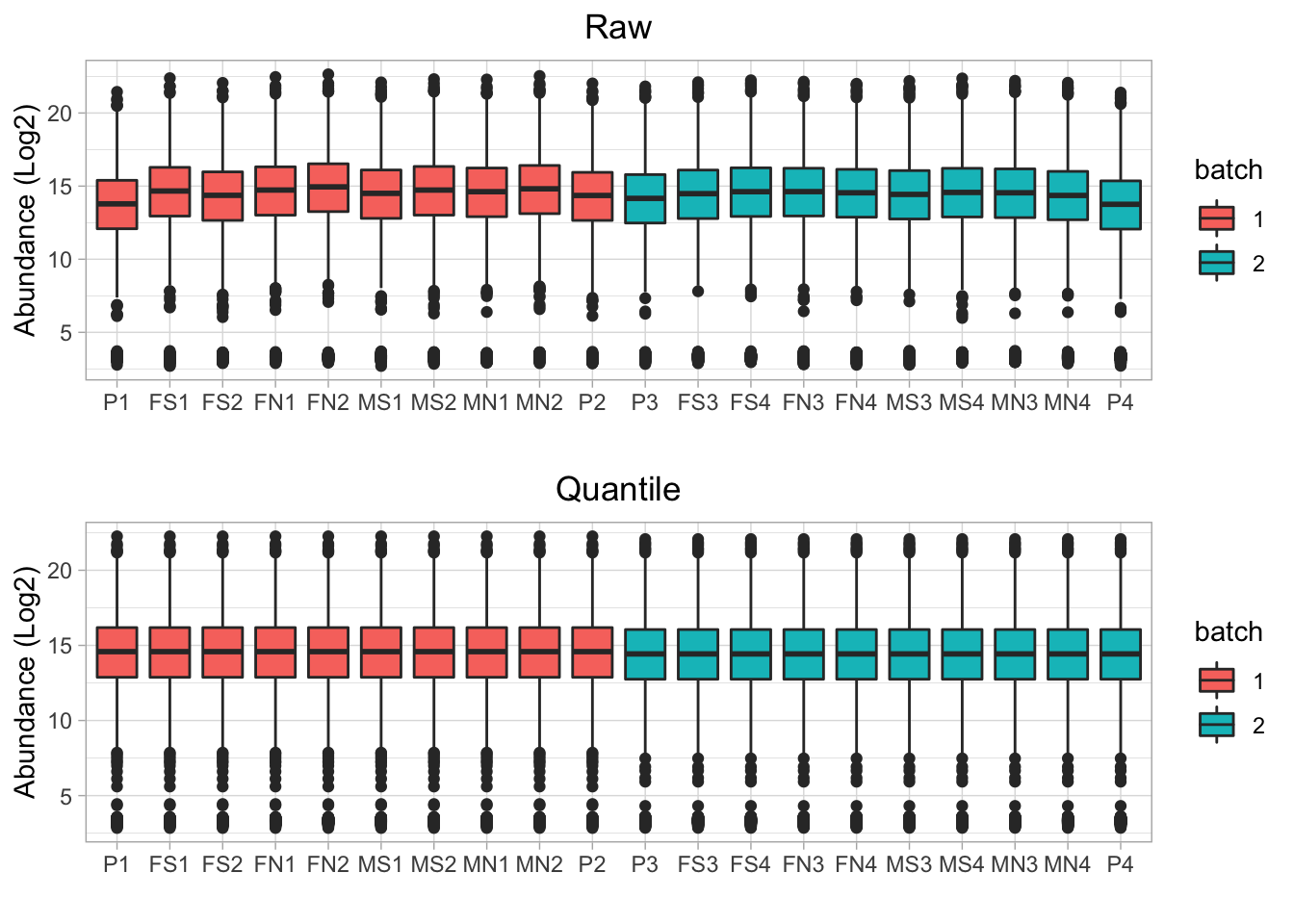
Figure 4.2: Boxplot of protein abundance for ech sample in mulitple batches (before and after normalization without batch effect correction)
After ComBat batch effect correction, the difference between the two batches is much smaller (Figure 4.3).
## Found 1 genes with uniform expression within a single batch (all zeros); these will not be adjusted for batch.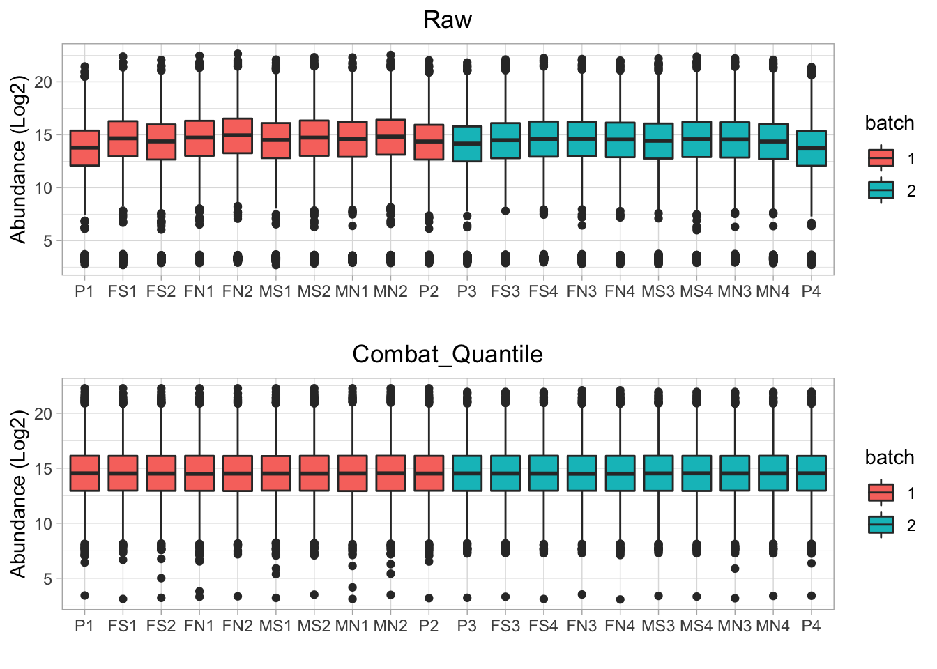
Figure 4.3: Boxplot of protein abundance for ech sample in mulitple batches (before and after normalization WITH batch effect correction)
4.2 Coefficient of Variation (CV)
Coefficient of variation measures the dispersion of data distribution. If a sample has multiple technical replicates, CV between these technical replicates should be small (ideally, CV should be 0). The samples in same situation, e.g. in control group, with same phenotype, should also have relatively small CV. CV of these technical replicates or samples in same situation can be used to check the performance of the data normalization.
Users can use cv column in sample information file to set the samples to calculate CV between each other. If column cv is not set, the samples with same sample.id (technical replicates) will be used to calculate CV. If there is no technical replicates and column cv is not set, all samples are used to calculate CV, which may not be a good mark to show the performance of the normalization. Please check Section 2.2 for details.
Figure 4.4 shows the CV between two technical replicates of raw data, after median and quantile normalization (example data for single batch).
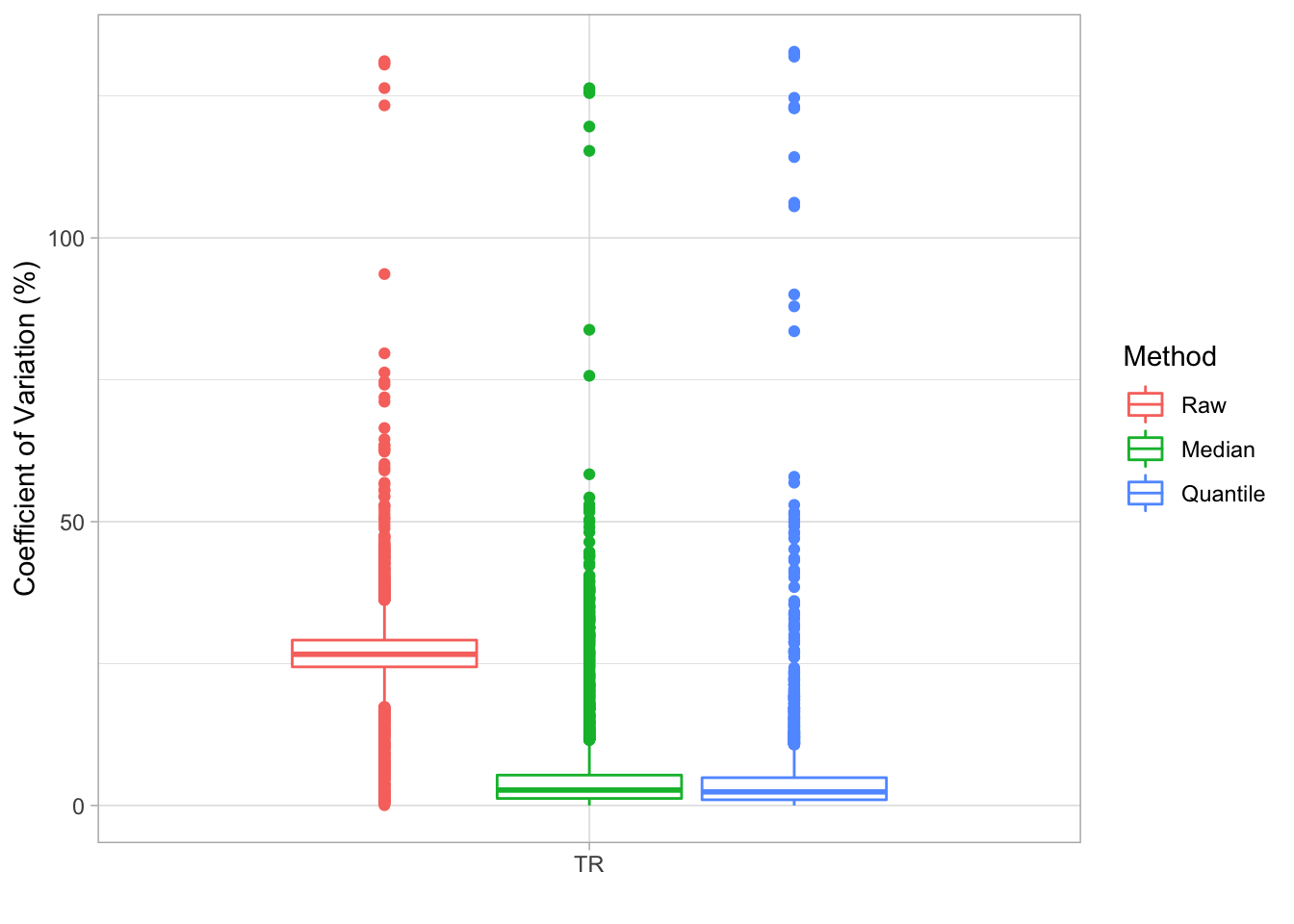
Figure 4.4: CV of technical replicates before and after normalization
Figure 4.5 shows the CV in each cv group, which is set in cv column of sample information file (example data for multiple batches).
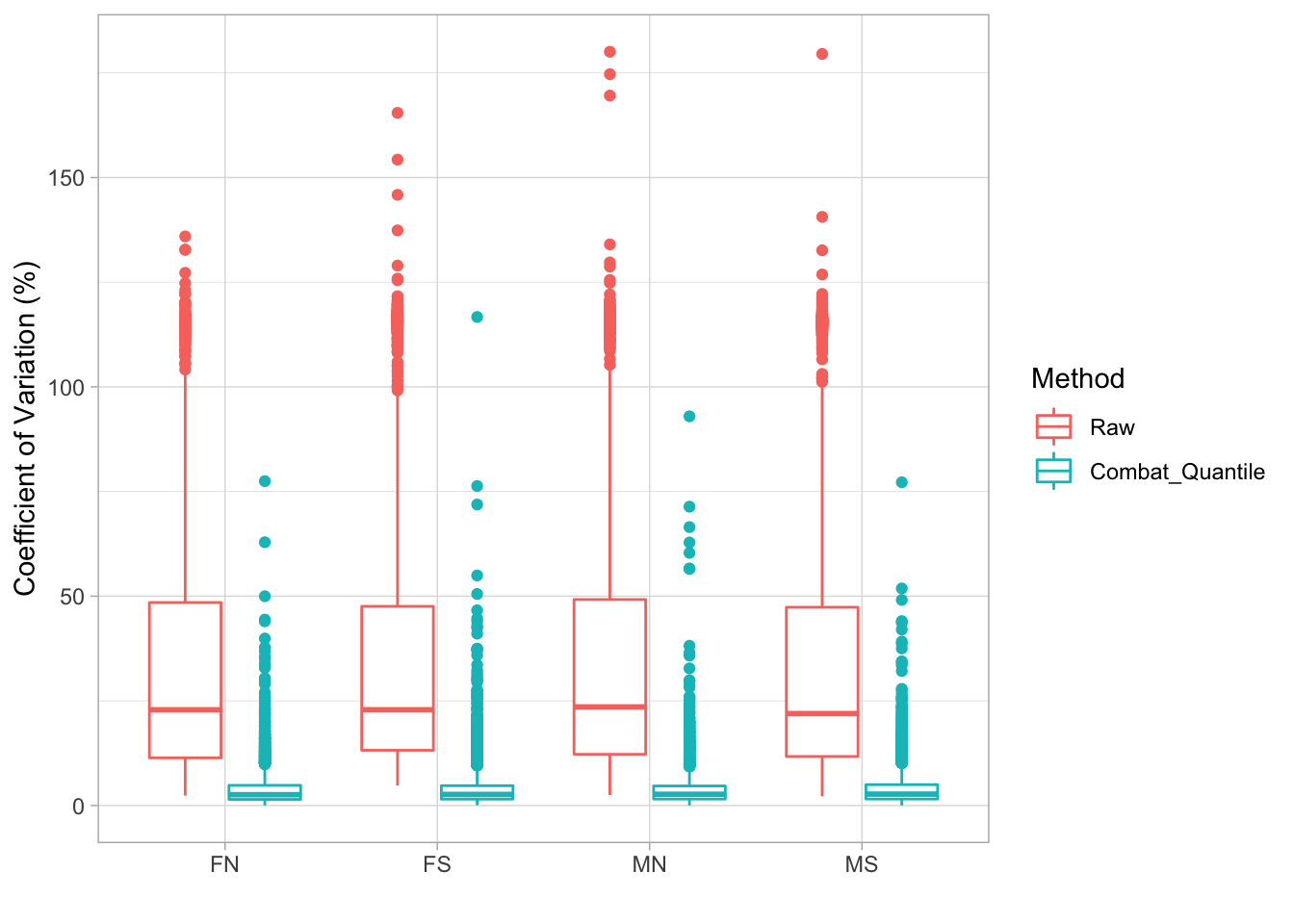
Figure 4.5: CV of samples in same cv group before and after normalization
4.3 Sample Clustering
Clustering method can also be used to choose normalization method. After data normalization, the technical replicates or the samples in the same condition should be clustered together (Ritchie et al. 2015).
Figure 4.6 shows the clustering result of raw data and the data after quantile normalization in each batch only. The samples in batch 1 are one the left of the figure and the samples in batch 2 are one the right of the figure, which indicates the large difference between the two batches. For the raw data, there is now clear cluster within each batch, while most similar samples in each batch are clustered together after normalization in the batch, e.g. FN1 and FN2.
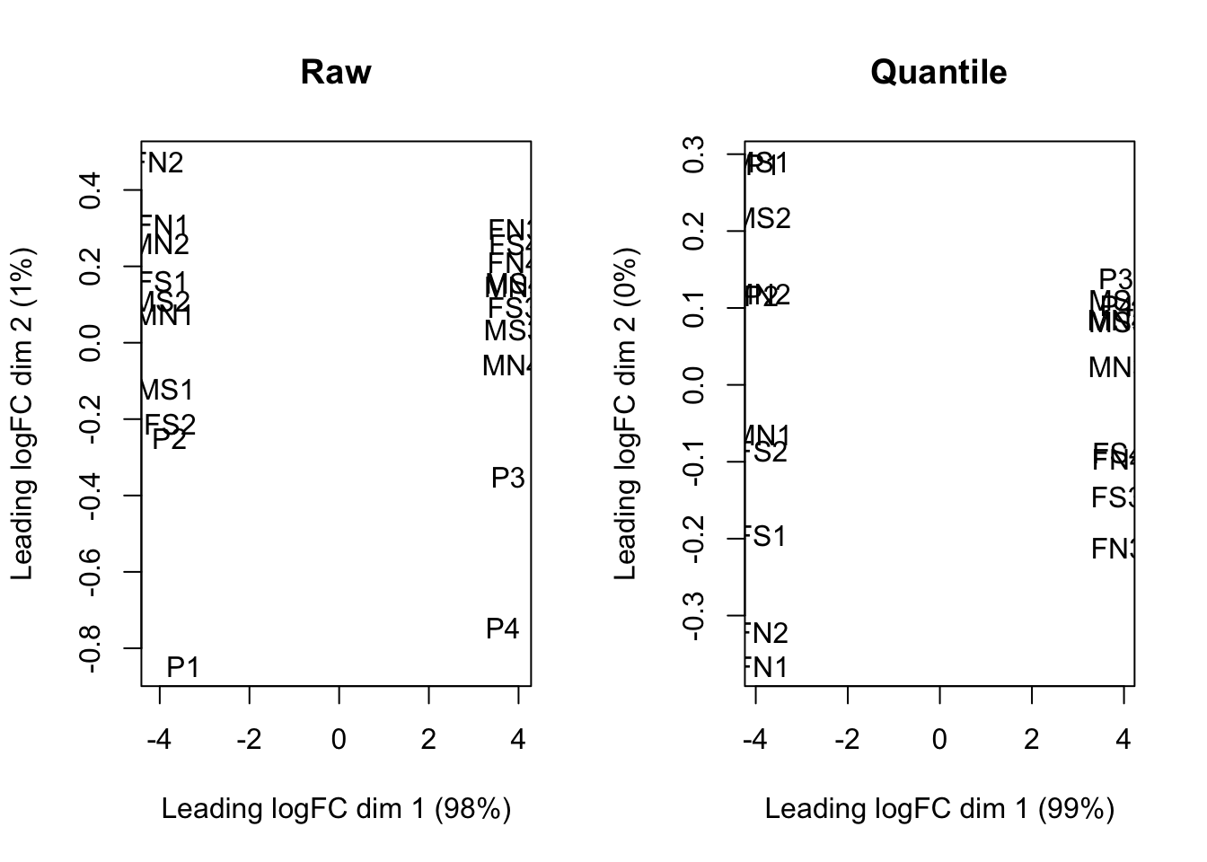
Figure 4.6: Cluster of samples of raw data and after normalization without batch effect correction
After both normalization and batch effect correction, the similar samples are clustered together even though they are not in the same batch (Figure 4.7).
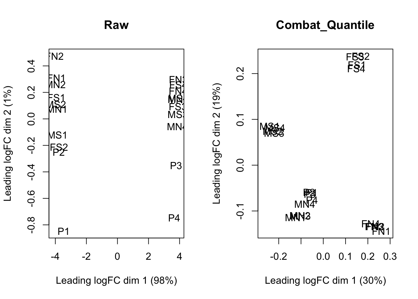
Figure 4.7: Cluster of samples of raw data and after normalization without batch effect correction
4.4 How to Choose Normalization and Batch Effect Correction Method
4.4.1 Boxplot
After normalization and batch effect correction, the boxplot should be similar to each other for all the samples.
4.4.2 Coefficient of Variation (CV)
Coefficient of variation between similar or technical replicate samples should be small, especially for technical replicates.
4.4.3 Sample Clustering
Similar samples should be clustered together. If there are no close connections between the samples, there should be no cluster groups.
4.5 Download Results
After checking the results after data normalization and batch effect correction, user can download the results by click Download Results button on the bottom of figures where users can select the normalization and batch effect correction methods.